Print That Beautiful Tableau Public Viz!! A 12-Step Guide

Over the past couple of years, I’ve spent some time on my newest hobby of running a dataviz themed sports shop on Etsy.com, which you can find here. The items in my shop were all created through the use of two tools; Tableau Public and Adobe Illustrator. Recently, several members of the community have reached out inquiring how I go about printing my visualizations. So, in addition to scheduling a BrainDate at Tableau Conference-ish about the subject of printing vizzes, I also wanted to write up a quick blog post that outlines the process. I’ve learned most of what I know today because of three people; James Smith, Eric Balash and Jeffrey Shaffer. My first inspiration came from stumbling across James’ beautiful Etsy shop, SportsChord, a few years ago. He has been extremely helpful in answering my questions and sharing his knowledge. Eric reached out earlier this year about getting an Etsy shop going. At that point, mine had very few items, all of which were being printed at a local shop I wasn’t overly impressed with. So, with the help of James, the two of us sort of set out on this journey together, learning a lot along the way, through trial and error. Check out Eric’s shop, Ready Set Data Prints. And Jeffrey’s blog post (see link below) has also been extremely helpful along the way.

So, the process outlined below is a process of printing Tableau Public visualizations I’ve found to work well for the needs of my Etsy shop. This process requires the use of Adobe Illustrator, but is by no means the only way to go about turning your Tableau Public work into a beautiful piece of wall art. Before we begin, I’ll point you to this important blog post by Jeffrey Shaffer in which he covers a variety of options explored during the making of “The Big Book of Dashboards.” If you prefer to not go through Illustrator, perhaps one of Jeffrey’s alternative options will suit your needs. Alright, let’s get started!!

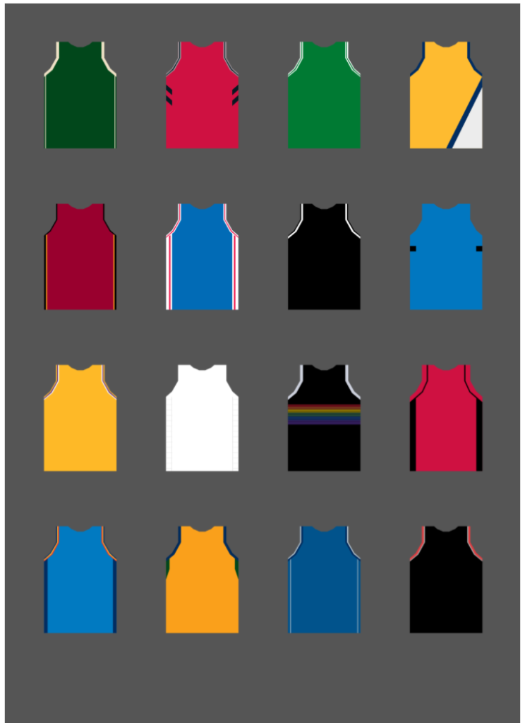
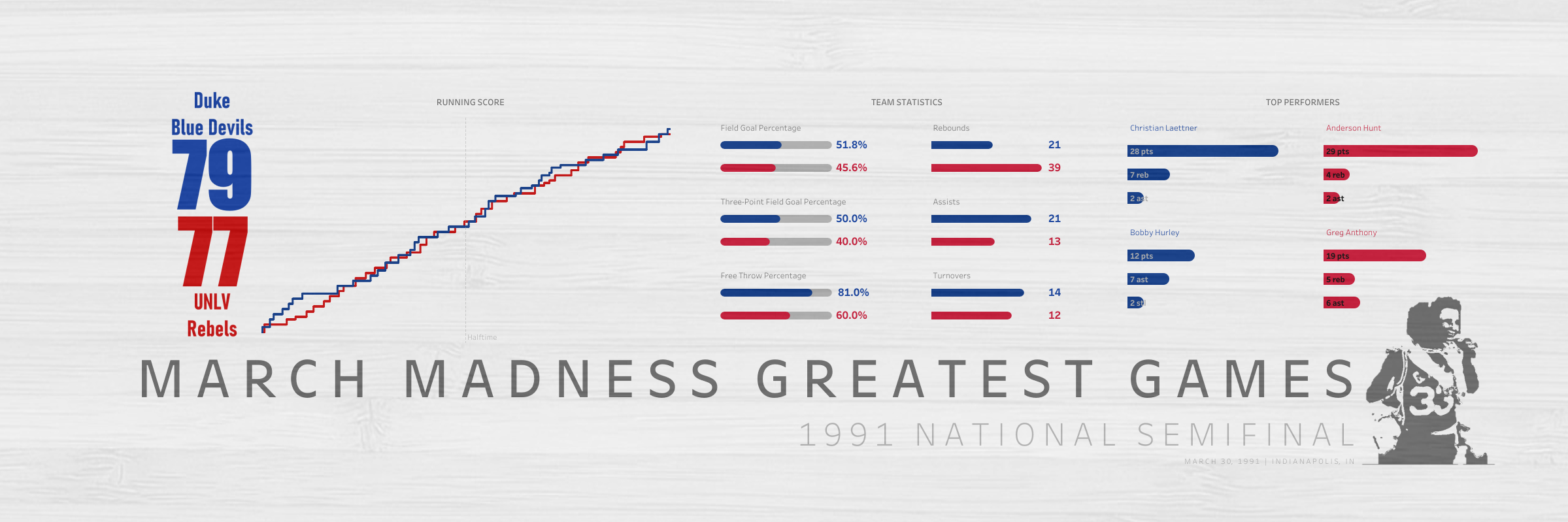
Step 1. Create a Tableau Public visualization– Create or identify the Tableau Public visualization you’d like to turn into a beautiful piece of wall art. Make the visualization the same size as the print you’d like to hang on your wall. For instance, if you’d like an 18×24″ print, make your Tableau dashboard 1800 pixels wide by 2400 pixels tall. Do not include any text in your viz, as we’ll use Adobe Illustrator to add the text in a later step. As we walk through the process, we’ll use my recent Black Lives Matter | 2020 NBA Playoffs viz as an example creating it at a size of 24×36″ (2400×3600 pixels). You can see the viz below with all of the text stripped out.

Note: For those skipping the Adobe Illustrator steps, leave the text in your Tableau Public visualization, refer back to Jeffrey Shaffer’s blog post, choose your desired method of creating a high resolution image and skip ahead to Step 9.

Step 2. Download Tableau Public viz as PDF – Download your Tableau Public visualization by clicking the download button on the bottom righthand corner of the page. A Download dialogue box will pop up. From the Download dialogue box, select PDF and then in the Download PDF dialogue box, change the Paper Size to Unspecified.

• 

• 

Step 3. Create new Adobe Illustrator project – Open Adobe Illustrator, select Create New and create an art board to the desired size of your print. In our example, we’ll create an art board with a width of 24″ and a height of 36″.

Step 4. Place the PDF into Illustrator – From the File menu, select Place and place the PDF into the workspace by clicking a blank space on the gray canvas.

• 

• 

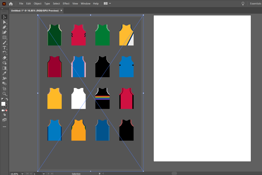
Step 5. Make Clipping Mask – From the toolbar select the rectangle tool and draw a rectangle (or square) over your print. DO NOT include the space between the outside of your viz and the blue line, as this is the PDF boarder we want to get rid of in this step. Once you have a nice precise rectangle drawn over your PDF, click on the selection tool and draw another rectangle, this time selecting both your PDF and the rectangle you just drew over it.

• 

• 

With both items selected, go to Object Menu -> Clipping Mask -> Make. This will complete the Clipping Mask, getting rid of that annoying PDF boarder.

Step 6. Place Image on Art Board – With the Selection Tool still selected, place your image on the art board by setting the X/Y coordinates to 0 and the W and H to the desired size of your print. 24×36″ in our case.

Note: when placing your image on the art board, there’s a little nine-square icon to the left of the X/Y coordinate boxes. This sets the reference point of your X/Y coordinates, so make sure the upper left box is white, otherwise setting X/Y to 0 will not work. You could also set the middle box as your reference point and then set your X/Y coordinates to the middle of your image; X = 12, Y= 18 in our example.

Step 7. Add text to your viz – Using the type tool, add text to your visualization.

Note: If you’re planning on creating a canvas print, you will want to add a 1.5″ boarder around your entire viz. This would be the portion of the canvas that is wrapped around the stretcher bar if you choose “image wrap” when placing your order. To do this, simply create a rectangle 1.5″ wider and 1.5″ taller than your print, with the same background color, then center your print on it. For our example, I’d create a 27×39″ rectangle with the same gray background. If your background is black, there’s no need for this extra step, as you can just select “black wrap.” when ordering from Prodigi.com. Lastly, if your background is not solid, you may want to make your original viz 1.5″ wider and taller, then leave that 1.5″ as extra spacing.

Step 8. Export as PNG – We’re now ready to export the image we’ll use for our print!! From the File menu, select Export and click Export As. Save the image to your desired location. Once you save, the PNG Options dialogue box will appear. Make sure the Resolution is set to High (300 ppi (pixels per inch)) and the Background Color is set to Transparent. Then click OK.

• 

• 

Note: Where you end up having your viz printed is definitely up to you, but I wanted to also include some steps to printing through Prodigi.com, the supplier who prints all of my Etsy orders. I first learned of Prodigi through a discussion with James Smith at TC19 and have been thrilled with their quality, turnaround time and excellent customer service. Learn more about their products here.

Step 9. Sign up at Prodigi.com and Create an Order – This is a pretty straightforward process. You’ll create an account, then sign in and create an order. Select the delivery country, paper/canvas type and size of your choice ( I use Enhanced Matte Art Paper for Posters and Standard Stretched Canvas on a Quality Stretcher Bar for Canvas prints).

Step 10. Add the image – Once you select the paper/canvas type, you’ll be prompted to add an image. Click Add Image, add your image and then click Edit Position. This will bring up a page that looks like the image below. Make sure your image is aligned and that the Quality is Excellent. Once you’re satisfied with the changes, click Save changes. That will bring you back to your Basket/Cart. From that page, click Continue.

Step 11. Enter your address – Next you’ll be prompted to enter your delivery address. Fill in the blanks and then click Continue.

Step 12. Submit your order – Next you’ll see a Summary of your order. Once you review it and everything looks good, click Submit Order!! Now, wait for that beautiful Tableau Public viz turned stunning piece of art to arrive at your door!! Note: Typical production time for Prodigi is 3-5 business days. Canvas will be longer than posters.

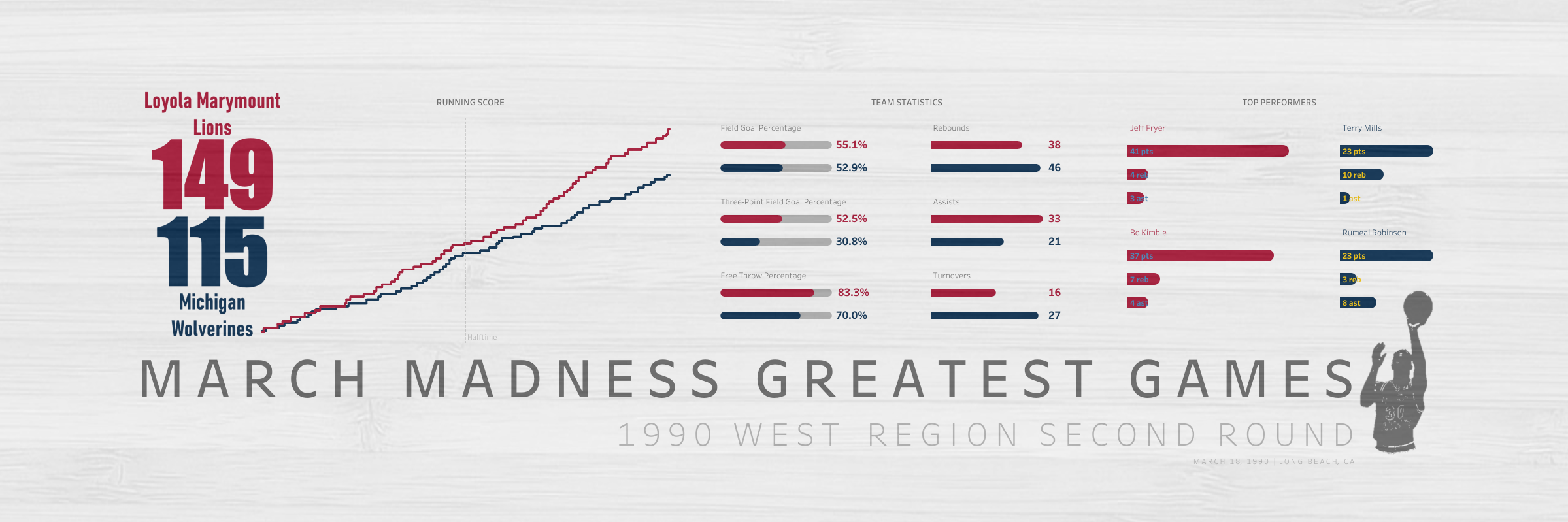
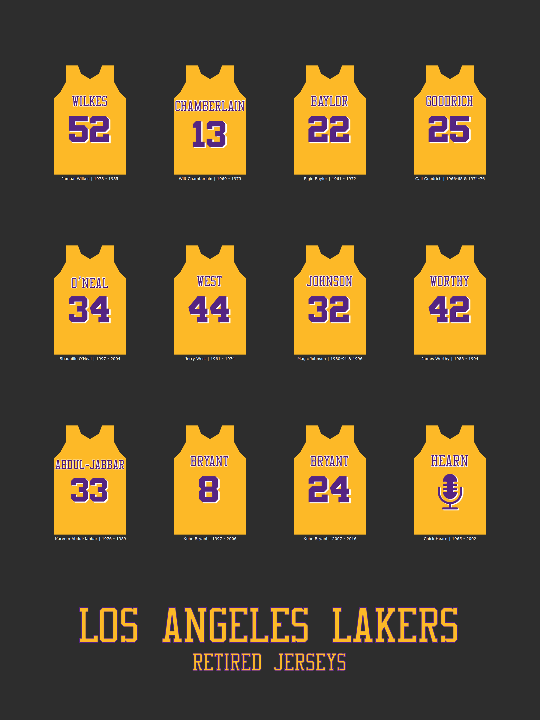
Hopefully this has been helpful and we start to see more tweets of beautiful dataviz wall prints in the near future!! And of course, if you have any questions please feel free to DM me on Twitter. Here are a few examples of visualizations of visualizations that have been printed. Thanks so much for reading and have a great day!!

Kobe Bryant Career Scoring Radial – Building the Viz

In late June, I published the Kobe Bryant visualization above after having been inspired by this beautiful Judit Bekker viz, ‘Moon Phases 2020.’ It had been well over a year since my last radial style visualization, so to aid in the building process, I reverse-engineered this awesome viz by Simon Beaumont, ‘Alan Shearer’s Premier League Goal Scoring.’ I was pleasantly surprised with how well the Kobe radial viz was received and was asked on several occasions if I would be writing a blog, sharing how the viz was created. So, while it should be noted that the creation of this viz would not have happened without the ability to download the vizzes by Judit and Simon or without amazing blog posts such as ‘Who’s Afraid of the Big Bad Radial Bar Chart? and ‘Beyond Show Me Part 2: Trigonometry’ by Kevin Flerlage and Ken Flerlage, I do feel it’s powerful to share what can be accomplished by downloading and reverse-engineering a viz from Tableau Public or by reading a blog post about a subject you may have avoided at all costs throughout high school and college!! So, let’s take a look at how I went about creating the Kobe Bryant Career Scoring radial chart.

The Data

After exploring Simon’s visualization a bit, it was clear I would need just two fields to build the radial lines for each season and a third field to size the dots that would be plotted around these radial lines. I had an old data set of Kobe’s career points by game laying around, because why wouldn’t I ;). So with the data ready to go, I was able to jump right into Tableau. Below is what the data looked like, with my key fields highlighted in yellow. In all reality, I could have built the entire viz with just these three fields, as the others were only used in tooltips, with the exception of Season ID, which was used for the bar charts…although I could have gotten away with using Radius for that, as it also corresponds to the Season ID.

Game ID and Radius would allow me to build the radials, while Pts would be used to size the dots

With the data pulled into Tableau, I was ready to get this show on the road, by building out a few calculations. Three calculations are needed to build the radial lines that the dots are plotted along. They are as follows;

1. An angle calculation for each of Kobe’s games played (called Game Angle)
2. X (to plot the x coordinates of each mark in the view)
3. Y (to plot the y coordinates of each mark in the view)

As we walk through the calculations in this post, I’ll do my best to explain what’s happening, but to gain a better understanding, I’ll again refer you to this fantastic blog post by 3x Tableau Zen Master, Ken Flerlage, titled ‘Beyond Show Me Part 2: Trigonometry.’

Game Angle – we need this to calculate X and Y, so we’ll start here.

To calculate the Game Angle, let’s first understand our spacing between each point (Game ID). Our Game ID field counts the games of each NBA season (a full NBA season is 82 games in length, so each season should have Game IDs running from 1 to 82). To figure out our spacing for a full circle we would take 360 (degrees in a circle) and divide that by the number of games in a season, which gives us 360/82 or 4.39 degrees between each point.

82 marks around the full circle, spaced 4.39 degrees apart

This spacing would work if our plan was to fill the entire circle. However, since we’re only using the first three quadrants of the circle and leaving the fourth quadrant blank, we need to push the spacing a little closer together. To do this, we replace 82 with 108, as this gives us the proper spacing (360/108 = 3.3333 degrees between each point) allowing Game ID 82 to fall right at 270 degrees. To get the proper angle for each Game ID we need to multiply Game ID – 1 by our spacing of 3.3333. For instance Game ID 1 would land at 0 degrees (0 x 3.333), while Game ID 2 would land at 3.3333 degrees (1 x 3.3333), Game ID 3 at 6.6667 degrees (2 x 3.3333) and so on.

82 marks around 270 degrees of the circle, spaced 3.33 degrees apart

Now that we have our Game Angle calculation, we can use it to calculate the values for X and Y. If you recall from reading Ken’s blog post, our Game Angle calculation will need to be converted to Radians, but we’ll just do that within each calculation. So, our X and Y calculations are as follows;

X = COS(RADIANS([Game Angle])) * [Radius]

Y = SIN(RADIANS([Game Angle])) * [Radius]

Building the Viz

We now have three of our four calculations needed to build the radial, so let’s walk through building it, together. We’ll begin by filtering Player to Kobe, as I’ve added other players to the data set since completing the Kobe viz. Now do the following;

1. Place X on the Columns shelf
2. Place Y on the Rows shelf
3. Drag Radius to Detail
4. Change the Mark type to Line
5. Drag Game ID to Path

You should end up with the below radial. However, we want Game ID 1 to start at 12 o’clock with the Game IDs moving in a clockwise direction as opposed to the current configuration, where Game ID 1 starts at 3 o’clock and Game IDs move counter-clockwise. To fix this, simply swap Rows and Columns and you’ll end up with the second of the two images below.

Before swapping Rows and Columns

After swapping Rows and Columns

Now that we have the radial lines for each of Kobe’s astonishing twenty seasons in the NBA, we’re ready to plot the dots that represent how many points he scored in each game. To add the dots, do the following;

1. Place Y on the Columns Shelf next to the existing Y
2. Create a Dual Axis
3. Synchronize the Axis
4. Hide the Headers
5. From the Marks card, change the second instance of Y to Circle

After changing the circle color to purple and increasing the size a bit, your viz should now look like the image below. We’re just about there!

Adding the dual axis and circle mark type

The only calculation remaining for the radial is the one that will color the dots according to how many points Kobe scored. For this calculation, I simply broke down his scoring into four groups, which you can see below.

After dropping this calculation on the Color card and setting our colors to Lakers colors, we’ll be left with the visualization below. I wanted all of Kobe’s 50+ point games to stand out, which is why they are colored white, with 10-49 point games colored in Lakers purple and yellow. Finally, Kobe’s games scoring less than 10 points, which occurred almost exclusively in the first couple years of his career, when he wasn’t getting much playing time, are colored a neutral gray. My two favorite parts of the viz are Kobe’s 2007 season in which he scores 50+ points in a stretch of five out of seven games, toward the end of the season, on his way to winning the NBA Scoring Title. The other is how clearly his 60-point career finale sticks out.

Placing our ‘Pts Color’ calculation on Color

And while this is a nice visual, it doesn’t quite do Kobe’s greatest games justice, so we’ll add the PTS field to Size and just like that, our radial is complete!! Now you can really see that 81-point outburst against the Toronto Raptors, on January 22, 2006.

Place PTS on Size and we have our radial!!

The only other parts of the visualization built in Tableau are the bar charts that show how many total points Kobe scored each season and the button for the information overlay.

The Printed Version

Since I knew this was a visualization I’d eventually want to print and add to my Etsy shop, all of the text was done in Adobe Illustrator to allow for a high quality print. Here’s the Kobe print as it appears in my shop. To celebrate the return of the NBA season, I’ll be running a 20% off sale beginning Thursday, July 30th through the NBA Finals for anyone interested in purchasing this viz or any other from the shop. Thank you so much for reading, I hope you found this post helpful and if you have any questions, please don’t hesitate to reach out to me on Twitter. Have a great day!!

Tableau Public Revizited | June 16, 2020

Tomorrow will mark ten years since Kobe Bryant won his fifth and final NBA Championship with the Los Angeles Lakers, defeating the Boston Celtics in Game 7 of the 2010 NBA Finals. This Tableau Public Revizited by Sekou Tyler provides an in depth look at Kobe’s legendary twenty-year career with the Lakers. Published by Sekou on March 14, 2020 I love the modern look and feel of this viz as well as the fact that I can quickly and easily get to game level data for every single one of Kobe’s 1,346 regular season games. Let’s jump in!

Three Things I Love!

Beautiful Design + Flow

Sekou’s viz leverages white space beautifully. The elements of the dashboard are well spread out, giving one another plenty of room to breath. This is crucial but can often be overlooked by developers. The purple ribbon on the left side allows the user to filter the remaining dashboard by season and on the top right side of the dashboard we have some key Kobe statistical categories; points, rebounds, assists and steals. Finally, the lower right section of the viz provides a trend of Kobe’s scoring over time, his top five scoring games, and game by game detail, all filterable by clicking on a season within the purple ribbon. The placement of each element by Sekou is well thought out and makes for a great user experience.

Great Interactivity

I had a lot of fun playing around in Sekou’s viz, filtering to different seasons, checking Kobe’s stats for each season and seeing what his top 5 scoring games were. I remember Kobe not getting a lot of playing time as a rookie, but didn’t realize it took him until his fourth NBA season to record his first 40-point game. Another touch I enjoyed checking out was the ability to filter a team from the Top 5 Scoring Games section to see all of Kobe’s games against that team for a particular season (or his whole career) in the Game Details section below. Kobe torched the Denver Nuggets during the 2002-03 season to the tune of 41 points per game, scoring at least 32 points in all four of his games against the Nuggets. I also noticed the Utah Jazz showing up A LOT on Kobe’s Top 5 Scoring Games list, so took to basketball-reference.com to do a little research. It turns out Kobe scored 1,549 points against the Jazz in 60 career games; 25.8ppg. However, if you throw out the first few seasons before Kobe became Kobe, you’re left with 1,328 points in 44 games or 30.2ppg. In one stretch from 2004 to 2009 Kobe scored the following in fifteen games against Utah; 34, 38, 40, 43, 30, 23, 27, 52, 35, 33, 28, 31, 27, 40, 37…simply incredible!

Game Details

As we touched on above, the Game Details section is great, especially for NBA nerds such as myself. It’s a necessary addition for the user to really be able to see the larger game-by-game body of work for Kobe. It’s also great for seeing the build up to probably my favorite Kobe moment of them all, his final game. In the week plus leading up to Kobe’s send off, he had been performing quite miserably, averaging just 17ppg on 32% shooting in the prior five games. So, to think Kobe would go off for even 30 or 40 points unlikely. But to surpass 50 points and then hit the 60-point mark was unreal. The Kobe haters would say “Yeah, but he took fifty shots.” But, you know what? Nobody cares…nobody cared then and nobody cares now, because NBA fans everywhere, Kobe supporters or not, were left with an unforgettable sports moment that will be remembered forever. If you have a few minutes to spare watch these highlights from the final 8:00 of that game. It’s a pretty special moment.

Big thanks to Sekou for a fun visualization. The design, cleanliness, flow and simplicity are top notch and I thoroughly enjoyed checking it out!! Great job Sekou, keep up the fantastic work!!

Tableau Public Revizited | May 27, 2020

It’s been far too long since our last Tableau Public Revizited, but time to get back to reviewing some great work of the past from the community we love so dearly. This week we’re looking at a nice viz by Kate Brown that I originally had lined up for Major League Baseball’s opening week. But, while we don’t yet know when we’ll be seeing baseball games again, we do know that this viz, ‘Enter Sandman,’ published by Kate back on March 30, 2019, captures the career of arguably the best closer the game has ever seen; Mariano Rivera. Let’s get to a few things that make this visualization so special.

Three Things I Love!

Clean Design + Just Enough Context

Kate starts out by doing non-baseball fans a big favor and providing some context. In her title header and again in the top left section of the viz, where readers eyes are drawn to first, she explains a little about Rivera’s career. As we touched on above, he’s one of the best closers the game has ever seen. However, when looking at the charts throughout the visualization, it’s important to know up front that Rivera began his career as a starting pitcher and then transitioned into the closing role after a few seasons.

This explains the high strikeout mark in 1996. In his set-up role, Rivera struck out a career high 130 hitters, but he also threw a career high 107 2/3 innings, nearly 30 more innings than his next highest season. So we would expect his strikeout totals to drop once he transitioned to the bullpen and began throwing closer to 60-80 innings per season. And without the note about his 2002 and 2012 injuries, readers would be wondering why so many of his stats took a dip both of those years. Looking at his stats on baseball-reference.com I can see that in 2002 Rivera pitched just 46 innings and only 8 1/3 in 2012. He threw at least 60 innings every other year he was the Yankees closer. So the context is very important and Kate does a great job of incorporating it into the viz while maintaining a clean design. Well done, Kate!

Use of Color

I really love how Kate uses just two colors (three if you count the white title) in the viz and ties them to team colors, the Yankees navy blue and gray. Also, the way she splits up the title and viz is nice, using the navy as the title background, but the gray as the background throughout the rest of the visualization. There’s no need for any additional colors.

Consistency

And speaking of a clean design, Kate’s use of bar charts throughout was a sound decision. She could have changed it up with different chart types, but why make it difficult for the reader to understand? Bar charts are easy to understand and the use of the same chart type for all five categories allows for easy comparisons across categories. For instance, Rivera enjoys his first 50 save season in 2001. If we look at the other categories, we can see how his strikeouts by season ramp up from 36 in 1998 to 83 in 2001. He also cut his walks in half, with just 12 walks in 2001 vs. 25 the prior season. More strikeouts and fewer walks is a great recipe for success.

What’s another great recipe for success? Do the things Kate did in this visualization. Clean, clear context, color, consistency. Oh and I also just love the image she chose. Great job Kate, this was a fun visualization to explore!!

Coming soon to History Visually on Etsy!

History Visually is an Etsy shop dedicated to capturing this history of great sports teams, careers and moments in visual form, printed and proudly displayed on your wall. While our shop currently offers four items, we have plans to add many more. See below for prints set to become available in 2020.

March Madness Greatest Games Collection | 36×12″ prints

1979 National Championship | Michigan State vs. Indiana State

1987 National Championship | Indiana vs. Syracuse

1990 West Region Second Round | Loyola Marymount vs. Michigan

1991 National Semifinal | Duke vs. UNLV

1992 East Regional Final | Duke vs. Kentucky

1994 National Championship | Arkansas vs. Duke

1997 National Championship | Arizona vs. Kentucky

2008 National Championship | Kansas vs. Memphis

2016 National Championship | Villanova vs. North Carolina

2019 South Regional Final | Virginia vs. Purdue

NBA Retired Jerseys Collection | 18×24″ prints

Los Angeles Lakers Retired Jerseys

Boston Celtics Retired Jerseys

…also stay tuned for the Philadelphia 76ers, San Antonio Spurs, New York Knicks and Detroit Pistons.

MLB Retired Jerseys Collection | 18×24″ prints

…also coming in 2020 are the New York Yankees, Boston Red Sox, Atlanta Braves, Cincinnati Reds, St. Louis Cardinals, Los Angeles Dodgers, San Francisco Giants, Pittsburgh Pirates, Minnesota Twins, Chicago White Sox.

 

Tableau Public Revizited | Mar 6, 2020

Published on March 7, 2018, this week’s Tableau Public Revizited is Explain Data before Explain Data! ‘Beautiful Billboard Bar Chart’ by Tableau Ambassador Sean Miller is an example of superb analysis and storytelling. Sean found a huge outlier in the data and dug in to find out what the cause was behind it. Let’s take a look at Sean’s work.

What makes this great data viz?

• Clear titles and annotations – In exploring Sean’s work, it’s clear to me he has read and taken away many learnings from Cole Nussbaumer Knaflic’s Storytelling with Data. His clear, descriptive title at the top of the page tells the reader exactly what question will be answered in the visualization below. Sean’s titles/text are consistent throughout the entire viz, helping the reader to easily understand what the visualization is telling them. He does an outstanding job in this area.
• Simple chart types – Another thing I like about the viz is the use of bar charts, a chart that is easy to understand and quick for readers to consume. In the first chart, the reader’s eyes are instantly drawn to the very tall blue bar at position 20. This is the focal point of the visualization and Sean pulls our attention directly to it. In the second chart, we can also see very quickly the spike in songs that spent exactly 20 weeks on the Billboard Hot 100, beginning in 1991.

• Use of Color – While the simple chart types themselves aid the reader in quickly understanding the story Sean is telling, his fantastic use of color helps drive it home. He begins with coloring the words “exactly 20 weeks” in the title with blue text, tying them beautifully to the data below that represents songs spending exactly 20 weeks on the Billboard Hot 100.

I wanted to share this visualization because it is an exceptional job of data storytelling. By combining the techniques covered above, Sean has taken a big outlier in the data and told the story behind it in a way that takes the reader only about 20-30 seconds to consume. Great job, Sean!

Tableau Public Revizited | Feb 18, 2020

As I sat down this afternoon, pondering which viz to feature in this installment of Tableau Public Revizited, my mind began to wander. I peered out the window into the frigid Minnesota temperatures outside, thinking of a place and time much warmer than the current 35-below wind chill. A place with lush green grass, sunshine, water and a warm summer breeze. A place perhaps, just like Chebeague Island, Maine.I’ve loved this viz, by Sue Grist, ever since I laid eyes on it. With its Jonni Walker-esque style it looks like something right out of a travel magazine. Let’s take a look at Sue’s beautiful piece of art.

What makes this great data viz?

• Beautiful Design – This map is so beautiful and I love how Sue sort of floats the text that provide more information about Chebeague Island in the waters surrounding the island. The grayed out shape of Maine with the blue dot representing Chebeague Island is a very nice, subtle extension of the title. I wouldn’t have otherwise known where, in Maine, Chebeague Island is, so this not only looks great, but is very helpful to the reader.
• Use of Color – The yellow dots on the map, indicating summer rentals, are great. I’m not sure how many colors Sue went through before landing on the yellow, but I played around with the viz a little bit and tried several other colors, none of which looked remotely as nice as the yellow she used. Tying the color of the dots to the text is best practice, so nice work there. Another thing Sue did really well was to set the opacity of the yellow dots to 65%. This lightens them up a bit and looks much more professional than if she had left the opacity at 100%. Just look at the difference in the image below.

Left: Opacity set at 65%         |        Right: Opacity set at 100%

• Ease of Use – Ok, we’ve covered the pure beauty of the visualization as well as Sue’s great use of color, but my favorite part about the ‘Maine: Visit Chebeague Island’ viz is the fact that I could see myself actually using it to plan a trip to Chebeague Island! It’s just so damn easy to use. In the bottom left-hand corner, Sue added a collapsible container where you can select your ideal summer rental based on numbers of bedrooms, bathrooms and/or how many people the unit sleeps. And then, while hovering over the yellow dots, we get a preview of the rental with the ability to navigate to the rental’s website, where we could book a trip right then and there.

So, which Chebeague Island rental was my favorite? Well, I’m glad you asked. I’d have to go with the Hackel Beach House at 47 Jenks Road. For me, this rental won out for several reasons, including its easy access to the beach and huge yard which is ideal for games like bean bags, croquet, bocce ball, etc. I also love the long deck that overlooks the ocean as well as the tongue and groove interior, which really gives it that cabin feel. Lastly, I definitely saw a fire pit in one of the pictures and you simply cannot have a summer cabin getaway without a bonfire to end the night!! While there’s plenty to do around the Hackel Beach House itself, biking around the island and ending up at the Slow Bell Cafe for lunch sounds like a good time. And when the kids are napping, maybe sneaking in a round of golf at the Great Chebeague Golf Club 🙂

It was a lot of fun exploring this viz in detail, Sue. Great job!

Tableau Public Revizited | Feb 4 , 2020

For the third installation of Tableau Public Revizited, we’re looking back at a powerful viz created by Kaleigh Piscioneri just over a year ago, on January 30, 2019. In her viz Kaleigh does an exceptional job breaking down the gender gap in sports. Let’s look at a few elements of this visualization that make it so effective.

What makes this great data viz?

• Use of Color – I absolutely love the colors Kaleigh uses in this viz and the faded gray is a perfect compliment to let that red really pop, grabbing the reader’s attention. The red is a powerful color to use here and is simple to understand. Anytime we see red in the viz, we know that color is associated with women, as Kaleigh ties it into the quote at the top of the page, as well as in a couple of other places. I can’t imagine a better use of color to tell this story. In my opinion, Kaleigh nails it!

• Chart Selection – The stacked horizontal bar charts at the top of the viz are nice as they do two things, aiding in the telling of the story while also separating the title from the rest of the visualization.
  • Unit Charts – The main focal point of the viz, Kaleigh’s use of the side-by-side unit charts is brilliant. The charts help drive home the disparity in earnings of professional male and female athletes better than any other chart Kaleigh could have placed here. We can quickly see that in 2017, of the Top 100 highest paid professional athletes in the world, just one was a woman. And in 2018, zero were women.
  • Donuts – Below the unit charts, Kaleigh looks more in depth at the difference in male to female average salary in three sports; basketball, soccer and tennis. The difference in basketball, where the average female salary is 1.3% that of the average male salary, is staggering to see visually. While soccer is not much better, tennis has far and away the smallest gap of the three sports. I like the use of donuts here, as it allows Kaleigh to add the KPIs in the center, while also including the background image to help the reader understand which sport is which.
• Tooltips – Upon first seeing the side-by-side unit charts, your initial thought is likely that you’re interested in knowing which athletes represent each of the dots. It’s a perfect use case for tooltips and Kaleigh does a great job of including more detail, as the reader hovers over a mark. While hovering on a mark, we can see that the female athlete who shows up in the 2017 Top 100 is Serena Williams. Name, rank, gender, sport, country and salary are all included in a very clean, compact layout. Nicely done! 

Exploring the viz – I was particularly interested to see which NBA players would show up each year. The reason being is that in 2015 the NBA salary cap was around $63 million, meaning each team could spend that amount of money on their roster, before being hit with penalties/taxes, if they exceeded that amount. By 2017, in large part to new TV deals, the cap had jumped to just north of $94 million, an increase of $31 million dollars from where it was in 2015. This led to teams over-spending on mid-level (average in terms of talent) free agents in 2017 and 2018, as they had the cap space to burn. Knowing this, I wanted to see how many of those mid-level players made the Top 100. After exploring the viz, I found five players who fit this description; Harrison Barnes, Chandler Parsons, Nic Batum, Steven Adams and Otto Porter Jr. were all among the Top 100, despite none of them ever being selected to an NBA All-Star game. While Batum and Parsons were making eight figures even before their new, free agent deals, the average salary of Barnes, Adams and Porter Jr. jumped from $4.3 million to an astonishing $23.1 million. Nothing like getting a near 600% raise for being just ok at your job!

Overall, I feel Kaleigh does a wonderful job of combining the elements we covered, to bring attention to this glaring gender gap in the earnings of professional athletes. Great viz, Kaleigh!

Tableau Public Revizited | Jan 20, 2020

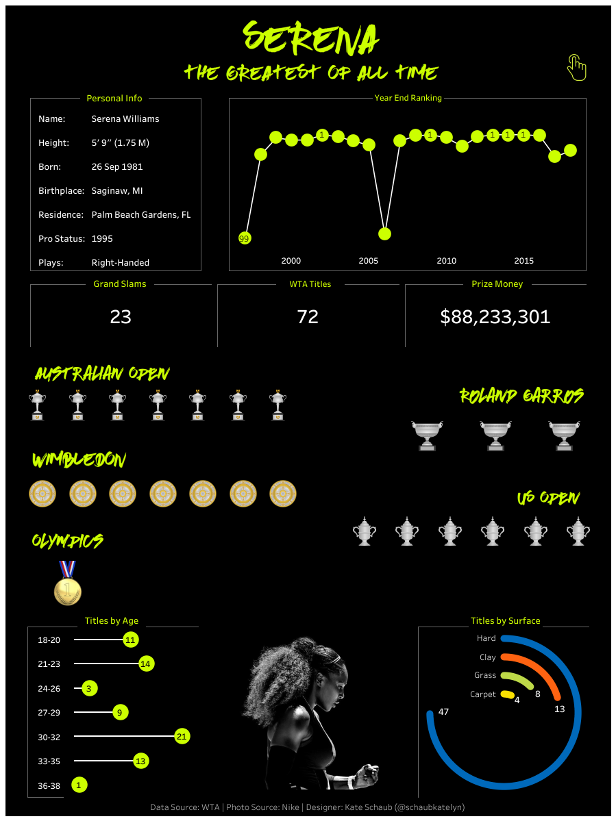
With 2020 Australian Open underway, this week we’ll be reviziting a beautiful viz from Kate Schaub, published on May 5, 2019. The viz, which has a really cool poster-like feel to it, is titled ‘Serena – The Greatest of All Time’ and it covers the amazing career of tennis superstar, Serena Williams. Let’s get started!First off, just take a step back and zoom out a bit to get a nice full shot of the viz. I really appreciate how well Kate thought through the design and layout of the visualization, as it flows together so well. Alright, let’s see what makes this a great data visualization.

What makes this great data viz?

• Design/Layout – As we just touched on, the visualization is laid out really well, in an order that makes it easy for the reader to follow.
  • Top section – this section features the title in an absolutely awesome font, while also including Serena’s personal information, ranking by year and some KPIs centered around her titles won and career earnings. Serena’s personal info in the upper left-hand corner is a nice touch, providing us with a little background on Serena Williams the person, before getting into Serena Williams, the tennis superstar. Next, we move onto year end ranking. Kate nails the chart choice here, given the theme, as the circles resemble tennis balls and the line chart gives the effect of the path of the ball. It’s amazing to see how many years Serena was ranked in the Top 7 (15 out of 22 years) and I also love how her 2006 ranking of 95th makes it look as though the ball is bouncing; very cool! Lastly, Kate includes some nice and clean KPIs that provide three key metrics; Grand Slam Titles, WTA Titles and Prize Money.
  • Middle section – After reading the KPI section, my first thought is what Grand Slams has Serena won and how many of each. I like the use of icons here displayed as unit charts, as seeing the actual trophy/medal Serena won adds a little something that we wouldn’t get had Kate gone with a plain circle or square in her unit chart. This also adds to the poster feel, I like it a lot. We can easily see that Serena’s won the Australian Open and Wimbledon seven times apiece, as well as the U.S. Open six times.
  • Bottom section – In this section, Kate provides more detail around Serena’s seventy-two WTA titles. The lollipop charts again give us the tennis ball feel and we can see that Williams started her career with a bang, winning twenty-five titles by the age of 23. However, her career appears to regress from age 24-29, which makes me wonder what happened? A quick Wikipedia search and it looks like Williams battled several injuries during this stage of her career. We then see her reaching peak dominance in her early to mid-thirties, before regressing again in her late thirties. This regression can be attributed to Serena’s pregnancy, which saw her miss almost the entire 2017 season. Lastly, I feel the image of Serena fits well in between the lollipops and the radial chart, which shows Serena’s titles won by playing surface.

• White Space – Kate does a really nice job of packing a ton of information into the viz, while not making it feel cluttered. She leverages white space to give each section of the visualization plenty of breathing room.
• Excellent Use of Color – Whether you see yellow or green, let’s just agree that the way the tennis ball color pops against the black background is a thing of beauty! Kate nailed it with this combination and another thing she did very well is to not overuse the large attention grabbing font. She placed it only where she wanted to guide the readers attention; beginning with the title and then the names of the Grand Slams, sticking with a smaller, more basic font for the other headers. She also uses the popping tennis ball color for the two main charts, very well done.
• Tooltips Provide Context – Tooltips are a powerful Tableau feature and particularly viz in tooltips, when used effectively. If we think back to Kate’s use of white space, we can see in the image below that her use of viz in tooltips helps prevent the viz itself from being cluttered. However, the tooltips pack even more insightful information into the viz. When I saw the viz for the first time, I remember thinking, “I wonder how many Grand Slams and how much Prize Money Serena has won compared to everyone else?” Well, wouldn’t you know, Kate included that very information through her use of viz in tooltips. The reader can also see who Serena defeated for each of her Grand Slams, as well as the score.

At the end of the day, this is a really cool visualization that should be framed and hanging on a wall somewhere. It’s pleasing to look at, designed very well and tells the story of one of the greatest athletes of all time. Great work, Kate!

Tableau Public Revizited | Jan 7, 2020

With over 750,000 Tableau Public authors and thousands of visualizations published daily, great visualizations are becoming more and more likely to fly under the radar. We’re most likely to remember the one that garnered thousands of views, a bunch of favorites and perhaps, even, a Viz of the Day. However, there are so many more visualizations on the Tableau Public platform that exhibit great data visualization skills. It’s for this reason that I’d like to introduce Tableau Public Revizited; a project dedicated to celebrating examples of excellent data visualization, which happened to fly a little under the radar, from a Tableau Public number of views standpoint. The only requirement to be considered for selection is that a visualization must have had fewer than 500 views on Tableau Public, at the time of selection. Ok, time to get started with our first visualization of 2020!

We’ll get Tableau Public Revizited underway with this fantastic viz from Justin Davis.Justin published this viz on October 23, 2019 and with the College Football National Championship game scheduled for Monday, January 13, what better time than now to highlight his viz? You may remember a visualization Justin created back in March, called ‘NCAA Basketball Salaries.’ That viz was recognized as not only March 28th Tableau Public Viz of the Day (#VOTD), but also as Tableau Public Viz of the Week for the week of March 25-29th. NCAA Football Salaries has the same layout, so I like the fact that we’re already familiar with the look and feel. Several elements make this a great Tableau Public visualization. Let’s take a look at the viz.

Justin’s visualization features the salaries of coaches from what are referred to as the ‘Power 5’ conferences of Division I-A college football; these conferences are the Atlantic Coast Conference (ACC), the Big 12, the Big Ten, the Pacific-12 (Pac-12) and the Southeastern Conference (SEC). The bottom right section also includes the Top 10 highest paid coaches from schools outside of the Power 5, including independent, Notre Dame.

What makes this great data viz?

• Simple layout – Grouping the bar charts by conference allows the user to quickly and easily compare salaries not only within each conference, but also across the different conferences. For instance, we can quickly see that Clemson’s Dabo Swinney and Alabama’s Nick Saban are the highest paid coaches in college football…and rightfully so, as these teams have combined to win the last four college football national championships, with two apiece. And furthermore, the only other team to even make an appearance in any of those title games was Georgia in 2017. Two other things grabbed my attention right away;
  • The fact that the highest paid coaches in the Pac-12 are paid quite a bit less than the highest paid coaches within the other Power 5 conferences.
  • Notre Dame’s Brian Kelly earns a salary of just $1.67 million. As a lifelong Irish fan, I’m aware of the fact that NBC has held Notre Dame football TV rights since 1991. And with the latest deal being worth $15 million annually, I assumed Kelly’s contract would be larger, so seeing it highlighted when I opened the viz, captured my attention.

• Clean formatting – You’ll notice the viz includes no grid lines and no axes. Why? Because, with the way Justin designed the viz, they are unnecessary. He includes a bar chart for each school and labels the value on the inside of the bar, which I love as well in this scenario. Not only does labeling the inside of the bar save some room, but it also allows the user to more easily scan down and read the salaries. It’s a much cleaner look than if he had labeled the ends of the bars. He also stuck with easy to read Tableau fonts which I’m a big fan of. Ok, now to my favorite part and the part that really makes this viz special, in my opinion.

• Effective Use of Color – Under the title, Justin includes a parameter driven slider, where the user can select a winning percentage of their choice. This then updates the visualization by highlighting coaches who have won at least that percentage of their games. The default is set to 85%, which is a great place to start. When I opened the viz, the first thing I did was slide it down to 50%, as I wanted to see which highly paid coaches failed to win 50% of their games. See the result below. We can see that Purdue’s Jeff Brohm and Florida State’s Willie Taggart were both paid at least $5MM and won fewer than 50% of their games. Taggart was actually fired by FSU earlier this season, after getting out to a 4-5 start, while Brohm is still hanging on as coach at Purdue, but had another disappointing year, finishing 4-8 this season.
  • One last really cool detail Justin added to the slider is dropping a calculation onto size that makes the 0%, 25%, 50%, 75% and 100% bands wider than the others. This helps make them much easier for the user to find. He also leverages a hover parameter action to drive the interactivity on viz itself.

All in all, I think this is a great example of a clean, effective visualization. Easy to understand, as we’re dealing with bar charts, not cluttered at all with any unnecessary text or labeling and powerful in its use of color. Great work, Justin!